
In short: Dissolved gas analysis reads the fault gases that oil and paper release when a transformer overheats or arcs. Since 2019 the IEEE guide has thrown out universal fixed limits and replaced them with 90th and 95th percentile values conditioned on transformer age and the O2/N2 ratio, plus two separate tables for how fast gas is moving. Levels tell you about the past. Rates tell you about now.
What is dissolved gas analysis?
Dissolved gas analysis is a laboratory test that measures the fault gases dissolved in a power transformer’s insulating oil. Electrical and thermal faults break the oil’s carbon-hydrogen and carbon-carbon bonds, and the fragments recombine into hydrogen, methane, ethane, ethylene and acetylene. Overheated cellulose adds carbon monoxide and carbon dioxide. The mix of gases can suggest a fault type. Concentrations and changes help decide whether to investigate, but do not by themselves establish severity or failure probability.
That is the whole idea. A transformer will not tell you it has a loose connection at a lead exit, but the oil around that connection will carry ethylene. The test is cheap, it is non-intrusive, and it has been the backbone of transformer condition assessment for sixty years. Interpretation requires the scope and conditions of the chosen guide, rather than an isolated limit copied from an earlier edition.
Which gases matter, and what does each one tell you?
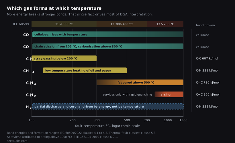
Seven gases carry the diagnostic load. IEC 60599:2022 clause 4.1 describes bond scission in oil followed by complex reactions in which unstable fragments recombine into gas molecules. Low-energy discharges favour hydrogen; higher energy or temperature favours other products. Breaking bonds in the original oil and forming the resulting gas molecules are distinct steps. The clause’s numerical discussion of these processes should not be reduced to a table of energies needed to break individual bonds in oil. Gas composition also depends on the reaction conditions and cooling history; molecular mass does not rank fault energy.
| Gas | What it points to | Formation mechanism and temperature |
|---|---|---|
| Hydrogen (H2) | Partial discharge, corona, stray gassing; also chemical reaction with galvanized steel | Low-energy cold-plasma discharges favour C-H bond scission and hydrogen accumulation as a recombination product (IEC 60599 cl. 4.1) |
| Methane (CH4) | Low-temperature heating of oil or paper | Heating of oil or paper (C57.104-2019 cl. 6.2.1). Present below 500 °C along with ethane |
| Ethane (C2H6) | Low-temperature thermal fault; stray gassing below 200 °C | A product of oil decomposition and recombination. IEC 60599 cl. 4.3 identifies H2, CH4 and C2H6 among the gases formed by stray gassing below 200 °C |
| Ethylene (C2H4) | Higher-temperature thermal fault, hot metal | Favoured over ethane and methane above approximately 500 °C, although also present in smaller amounts below that temperature (IEC 60599 cl. 4.1) |
| Acetylene (C2H2) | Arcing, high-energy discharge | IEC 60599 cl. 4.1 describes formation at high temperatures, approximately 800 °C to 1200 °C or above, followed by rapid quenching for accumulation as a stable product. Significant quantities are associated mainly with arcing; much smaller amounts can form below 800 °C |
| Carbon monoxide (CO) | Cellulose degradation; also oil oxidation | Paper chain scission becomes significant above 105 °C, complete carbonization above 300 °C (IEC 60599 cl. 4.2). Oil oxidation also yields CO over long periods (cl. 4.1) |
| Carbon dioxide (CO2) | Cellulose degradation, ageing, oxidation | Same cellulose route as CO. Formation rises with temperature, with oil oxygen content, and with paper moisture (IEC 60599 cl. 4.2) |
Two cautions on the carbon oxides. C57.104-2019 states in Annex D.8 that CO is not always a good indicator of a fault in paper, so a raised CO/CO2 pair on its own is weak evidence. Hydrogen also has non-fault sources, including chemical reactions and stray gassing. An isolated rise needs investigation in context; it should not simply be dismissed.
What actually changed in IEEE C57.104-2019?
The 2008 edition gave you one table of fixed concentration limits and a TDCG number. Both are gone. The 2019 revision removed TCG and TDCG from its current interpretation procedure, retaining earlier material for historical reference in Annex G, and it moved Doernenburg and Key Gas out of the main text into an informative annex. In their place sits a statistical model built on approximately 1.5 million DGA samples.
The reason for the change is worth stating precisely, because it is the part most summaries skip. Two variables turned out to shift the typical gas population substantially: the O2/N2 ratio, used to distinguish gas populations associated with different oxygen conditions, and transformer age. In the dataset used to develop Tables 1 and 2, rating, voltage class and oil volume did not contribute significantly to the selected concentration values, so those tables were not subdivided by them. Their influence was not studied for Tables 3 and 4. This does not establish that they are irrelevant in every fleet; clause 6.1.2.5 warns that gas populations can differ with these and other asset characteristics. A single universal limit for hydrogen is therefore a compromise between populations that genuinely behave differently. It is not a physical threshold.
Read clause 6.1 carefully and you find something else. The guide classifies DGA results, not transformer condition. C57.104-2019 says users should not equate DGA status to transformer condition, and it notes that transformers can fail with no prior gas generation while others run for years at high levels. This is a statistical screen, not a verdict.
What counts as low, and what counts as high
The guide sets two reference levels for every gas: a 90th percentile below which the gas counts as low, and a 95th percentile above which it counts as high. The tables distinguish O2/N2 populations and include age bands where relevant. The ratio does not reliably identify a particular transformer as sealed or free-breathing; clause 5.4 explicitly cautions against that inference. The values themselves are published in the standard and we do not republish them here. What the change means in practice, and why a limit needs its edition and application conditions, is covered in our guide to normal dissolved gas levels in transformers.
The conditioning is the whole point. For ethane in the O2/N2 ≤ 0.2 population, the level that counts as low in a transformer under ten years old is roughly a fifth of the level that counts as low in one past thirty. Same gas, same guide, same page. Apply the lower young-unit value to older units and you can create additional flags; apply the higher old-unit value to young units and you can miss an unusual increase. The direction matters. Age and oxygen conditions are part of the screening rule.
The tables are also worth reading for their irregularities. Percentiles built from field data are not always monotonic with age, and at least one cell runs against the trend of its own row. That is what happens when a limit is measured rather than decided, and it is a good reason to treat any single cell as a screening aid rather than a verdict.
Status 1, 2 and 3
Three classifications, defined in clause 6.1. Status 1 covers low gas levels with no indication of gassing, described as unexceptional. Intermediate levels or possible gassing put a unit in Status 2, possibly suspicious. High levels or probable active gassing put it in Status 3, probably suspicious. Tables 1 and 2 set the level boundaries. Table 3 defines possible gassing, Table 4 defines probable active gassing.
Clause 5.4 is candid about what this costs. If any one gas above a norm flags the sample, the guide expects roughly 40% of all DGA results to need further review once Tables 1 and 3 are both in play, and about 20% to land in Status 3 once Tables 2 and 4 are combined. These are population-level expectations, not measured false-positive rates or a forecast for every fleet. Clause 5.4 notes that a smaller or different population may yield different proportions and that programmes need resources for the resulting reviews.
Why rate of change became a first-class test
This is the genuinely new machinery, and it deserves more attention than it gets. Table 3 gives the 95th percentile of the delta between two consecutive laboratory samples, with no normalisation for elapsed time. Its companion, Table 4, holds the 95th percentile of rates from a 3-to-6-point linear regression in ppm/year, with norms derived from samples whose gas levels sit below Table 1. That describes the reference dataset, not a ban on calculating rates at higher concentrations; clause 6.1.1 also uses rate information in later screening steps.
Note what the standard says about the first of the two. It is dominated principally by fluctuation from the analysis process itself, not by the transformer. It is a noise floor. When concentrations remain below Table 1 but a delta or rate norm is exceeded, clause 6.1.1 Step 4b calls for a confirmation sample within one month. Other results and operating evidence can require a different response.
Acetylene is the exception in both tables: the entries are any increase and any increasing rate. This warrants careful review, including analytical uncertainty. It is not proof of main-tank arcing. IEC 60599:2022 clause 4.4 describes residual acetylene from manufacturing or welding in new stainless steel, and a communicating tap changer can also contaminate main-tank oil.
How does IEC 60599 assign a fault type?
Where the IEEE guide screens, IEC 60599:2022 classifies. Clause 5.4 uses three basic gas ratios to sort a fault into six classes, derived from internal inspection of hundreds of faulty units. The physical definitions come from clause 5.3: thermal faults below 300 °C leave the paper brownish, above 300 °C it has carbonised, and above 700 °C you see oil carbonisation, metal coloration around 800 °C, metal fusion above 1000 °C.
From IEC 60599:2022 Table 1, decimal commas as printed. Two footnotes carry real weight in practice. For partial discharges in instrument transformers the CH4/H2 threshold moves to 0,2, and in bushings to 0,07. On the T3 row, a rising acetylene content indicates a hot spot above 1000 °C.
The standard admits its own overlap. D1 and D2 share territory, so a dual attribution is sometimes the honest answer, and the distinction survives only because the energy involved changes what you should do about it. Ratio combinations falling outside every range get no diagnosis at all. That happens more often than the tidy table suggests. Clause A.2.3 adds a trap worth knowing: on a transformer with a communicating OLTC, a C2H2/H2 ratio above 2 to 3 can indicate contamination from the tap changer. Table 1 should then be avoided or used with care, with the effect of contamination assessed; subtracting an unknown background would create another unsupported result.
How do you read the Duval Triangle?
Duval Triangle 1 uses three gases ordered by the energy of the fault that makes them: methane for low energy, ethylene for high temperature, acetylene for arcing. Take valid, non-negative concentrations in ppm, check that their sum is positive, then express each as a percentage of that sum. A zero total has no defined position. Those three percentages are the coordinates. C57.104-2019 clause D.4 gives the arithmetic: with x for acetylene, y for ethylene and z for methane, %CH4 = 100z/(x+y+z), and likewise for the other two.
The zone boundaries are defined in C57.104-2019 Table 6. The DT zone covers mixtures of electrical and thermal faults, which is why the standard needs three separate boundary rows to describe it. The diagram below illustrates those boundaries; the numeric grid belongs to the standard and stays there.
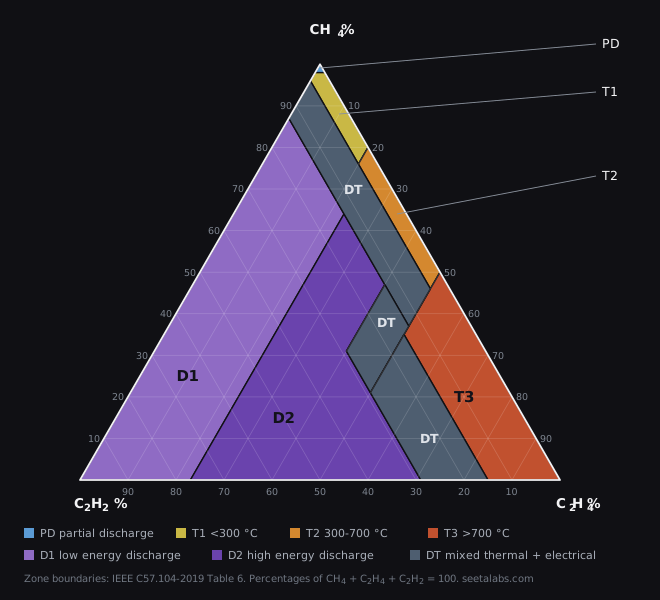
The triangle’s strength is that it always returns an answer, since normalised percentages must land somewhere inside it. That strength is also the trap, and C57.104-2019 says so in as many words: because it always gives a diagnostic, it should be used only when other information indicates a fault is likely to exist, and identifying a fault type is not itself confirmation that a fault exists. Feed it three trivial numbers and it will confidently name a fault. How to read the triangle properly, what each of the seven zones implies for the asset, and where the method stops being trustworthy are covered in our guide to the Duval Triangle.
When Triangle 1 lands on PD, T1 or T2, Triangle 4 (H2, CH4, C2H6) resolves the low-temperature sub-types including stray gassing. For T2 or T3, Triangle 5 (CH4, C2H4, C2H6) separates the high-temperature sub-types. Neither Triangle 4 nor Triangle 5 should refine a D1 or D2 result. Duval Pentagon 1 uses hydrogen and four hydrocarbon gases at once, centre at (0, 0) and the H2 apex at (0, 40), covering the same six fault classes plus stray gassing. Running a pentagon and a triangle side by side has a specific use: a disagreement can indicate multiple simultaneous faults, as discussed in clause D.7, but needs engineering interpretation and is not proof of multiple defects.
Are Rogers ratios and Key Gas still worth running?
Short answer: as a cross-check, not as your primary method. The 2019 revision places Key Gas and Doernenburg in Annex D and retains Rogers in clause 6.2.2. The guide describes limitations that matter when selecting or cross-checking a method.
The guide states the limitation of the Rogers scheme immediately after publishing it: the method fails to identify a fault in typically 35% of DGA results, because they match none of its cases, and this happens even when concentrations are high and a fault is obviously present. One sample in three comes back empty.
Key Gas is worse. Clause D.1 puts it at typically 50% inconclusive or wrong identifications when applied automatically in software, dropping to typically 30% when an experienced engineer applies it by hand. A method that is wrong or silent half the time under automation has no business driving a fleet screening pipeline. It survives because it is easy to teach, and because the underlying intuition, that the dominant gas hints at the fault, is sound even where the formalisation is not.
Why do ratio methods fall apart at low concentrations?
This is where most people get it wrong, and it is the cleanest test of whether someone understands DGA or is reciting it.
Every ratio method divides one small number by another small number. When both sit near the detection limit, the quotient is dominated by measurement error. C57.104-2019 clause 5.2.1 draws the line explicitly: below about five times the method detection limit, a few ppm depending on gas and method, relative measurement uncertainty can be large, and fault identification or practical decisions should not rest on such values without confirming their accuracy. The same clause generally advises against fault identification when every gas lies below Table 1. It allows experienced users to apply additional rules with caution where concentrations exceed about five times the detection limit; that exception is not a licence to interpret arbitrary low values.
Laboratory accuracy is not what people assume either. IEC 60567 recommends better than ±15% to avoid misidentifying faults. C57.104-2019 records that several laboratories meet that requirement and several others do not, with measurement errors as high as ±60% or more for some gases. Sixty percent. Divide one gas carrying that error by another and the result is arithmetic theatre.
Acetylene deserves its own warning, and the standard gives it one. Where acetylene is the only gas above its screening level but still below five times the detection limit, clause 5.2.1 says fault identification in that case may be unreliable. Confirm the accuracy of that result and obtain further evidence. Resampling can help, while urgent operating or protective decisions must also consider the other signs of a developing fault.
Why does the trajectory beat the snapshot?
Clause 5.4 makes an argument that ought to be printed on the wall of every asset management office. High gas levels suggest an eventful past. A transformer with twice the gas level of another is not twice as likely to fail. Stable gas, even at high concentration, is history. Active gas formation, even at low concentration, means something is happening now.
The arithmetic of naive rate calculation is where the trouble starts. C57.104-2019 works an example that is hard to argue with. Take two consecutive samples differing by 2 ppm purely from analytical variability. A year apart, that computes to 2 ppm/year. Shrink the interval to a month and the same 2 ppm reads as 24 ppm/year. One day apart, 730 ppm/year. Same physical transformer, same non-event, three answers spanning more than two orders of magnitude, driven entirely by when the technician happened to visit.
The fix explains why Tables 3 and 4 exist as separate instruments. Data analysis showed that the delta between two consecutive samples is mostly unrelated to the time between them, about the same for samples a week apart as for samples two years apart, which makes percentiles of simple time-normalised rates unusable. So Table 3 drops time normalisation entirely and asks only whether the step exceeded analytical noise. Table 4 then uses three to six points and linear regression, because random analytical variations tend to cancel across multiple samples, leaving actual transformer gas evolution behind.
For the multipoint procedure, clause 6.1.1 Step 2 specifies three to six points over the last four to twenty-four months. Its note, and Step 5, state that one sample per year does not provide enough points for the Table 4 comparison; Step 5 uses Table 3 in that case. If its delta values are exceeded, a confirmation sample can supply the additional point needed, with three samples in two years given as an example. Check the actual sample dates and any additional follow-up measurements before deciding whether a valid multipoint series is available. If you are working out where your own fleet sits on that curve, a structured fleet-wide DGA screening pass will show which units have enough history to trend and which lack enough dated observations for that trend calculation.
What does DGA not see?
Any honest treatment has to include this section, and most vendor material does not. Main tank DGA sees faults that vent gas into main tank oil. Several important failure populations do not.
C57.104-2019 clause 6.1 puts the boundary plainly: DGA should not be assumed to replace other prudent operating, management and monitoring practices, and conclusions should never be based exclusively on a single DGA result. Any tool claiming to score transformer health from oil gases alone is scoring a fraction of the failure modes. Ours included, which is why a score should always arrive with its confidence and its blind spots attached rather than as one unqualified number. How we present that is described on the RONIN platform page.
How often should you sample, and what do you do at each Status?
C57.104-2019 deliberately publishes no universal sampling interval. Routine frequency is left to company policy or the manufacturer’s recommendations, and the guide repeats that at every Status. What it does specify is the structure around those samples.
For a new unit, a repaired unit, or one whose history was reset by oil processing, clause 5.3.1 recommends a sample before and during commissioning, then several more over a few weeks to a few months after energisation to establish a baseline. Manufacturers often supply their own norms during warranty, typically tighter than Table 1.
For routine screening the computation each time is: O2/N2 ratio, absolute delta against the previous sample, and multi-point rates over the last three to six data points spanning four to twenty-four months. Where more than six points exist, clause 6.1.1 Step 2 says use the six most recent, not exceeding two years.
What follows from the classification:
Two habits separate programmes that work from programmes that generate noise. Confirm surprising or alarming results with another sample where practical, as clause 6.1 advises. Do not delay urgent protective action when other operating evidence warrants it. Then compare against sister units built to similar specifications, which clause 6.1.1 recommends for spotting unusual results and revealing common patterns.
One last caution for anyone installing monitors. Under continuous monitoring, clause 5.3 states that the screening norms no longer apply, particularly the rate norms, and that higher rate values than laboratory DGA are commonly used. Apply Table 4 to a monitor sampling four times a day and you can create inappropriate alarms because the sampling process and rate calculation have changed.